Understanding BigQuery Editions, a practical guide
How to balance price and performance the right way
First and foremost, I want to thank to my colleagues and friends, Amine and Sabri, for their sharp eyes in reviewing this!
Introduction
In the ever-evolving tech landscape, trends come and go but some things age gracefully and prove durable: BigQuery is approaching its 15th anniversary 🎉
A lot has changed along the way (BigQuery ML, Analytics Hub, BI Engine, BigQuery Omni), but the product has stayed focused on its original promise: querying data at scale in seconds without the overhead.
If you already know everything about BigQuery and just want to see the case study, directly jump here.
Since day one, BigQuery’s pricing has reflected its architecture, separating compute from storage. Storage is priced by the amount of data stored and compute costs can be billed in two different ways, depending on the model chosen:
On-demand
There’s no data warehouse to create and to size, no warm-up time and nothing to shutdown after — you just write and run your query, as simple as that. You’re billed by the amount of data processed by each query, pay-as-you-go for data processed. We are gonna run all ours tests in US multi-regions, with a cost of $6.25 per TB. This offers unmatched ease for starting new use cases when you don’t know much about your usage patterns. Additionally, you can set daily or per-user spending limits to ensure controlled costs and prevent any unexpected overruns.
Capacity-based
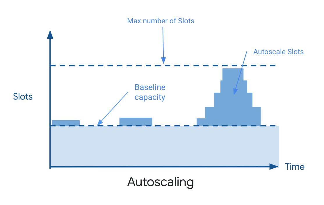
You purchase dedicated capacity at a fixed cost. Choose the right price-performance for individual workloads needs with the ability to adapt and allocate capacity to each workload. This model is called BigQuery Editions, with three different editions tailored to your feature needs. Both models rely on the same notion: slots. A BigQuery slot is a virtual worker node used by BigQuery to execute SQL queries. During the query execution, BigQuery automatically calculates how many slots a query requires, depending on the query size and complexity. With a capacity-based model, you can pay for dedicated or autoscaled query processing capacity. The capacity-based model gives you explicit control over ratio cost/of cost to performance for each business case or environment. (More information is available here)
A good rule of thumb for choosing between the two is, for a given workload: start with on-demand billing, then switch to a capacity based approach once your usage stabilizes. To that extent, high query volume (QPS) often justifies using an Edition for better cost-efficiency. Keep in mind that you can use both on-demand and Editions concurrently for different workloads, and freely switch between them as needed.
A good rule of thumb for choosing between the two is, for a given workload: start with on-demand billing, then switch to a capacity based approach once your usage stabilizes. To that extent, high query volume (QPS) often justifies using an Edition for better cost-efficiency.
Keep in mind that you can use both on-demand and Editions concurrently for different workloads, and freely switch between them as needed.
CASE STUDY
Having laid the groundwork, let’s move to a practical case study. Here, we’ll compare the same query running on-demand versus using an Edition to illustrate why we recommend starting with the former and transitioning to the latter. Let’s start by creating a BigQuery reservation:
CREATE RESERVATION
  `PROJECT_A.region-us.bqe-tests`
OPTIONS (
  edition = "ENTERPRISE",
  autoscale_max_slots = 200 );
First use-case: the scarce query
The first use-case is a (on-purpose) complex but scarce query, calculating the average page views of Google’s Wikipedia article on the first day of January, February, March, and April 2024. With more than 90M records, the table is around 1.50TB. Our query is fetching around 30GB of data:
WITH
january_first_views AS (
  SELECT * FROM `bigquery-public-data.wikipedia.pageviews_2024`
  WHERE TIMESTAMP_TRUNC(datehour, DAY) = TIMESTAMP('2024-01-01')
),
february_first_views AS (
  SELECT * FROM `bigquery-public-data.wikipedia.pageviews_2024`
  WHERE TIMESTAMP_TRUNC(datehour, DAY) = TIMESTAMP('2024-02-01')
),
march_first_views AS (
  SELECT * FROM `bigquery-public-data.wikipedia.pageviews_2024`
  WHERE TIMESTAMP_TRUNC(datehour, DAY) = TIMESTAMP('2024-03-01')
),
april_first_views AS (
  SELECT * FROM `bigquery-public-data.wikipedia.pageviews_2024`
  WHERE TIMESTAMP_TRUNC(datehour, DAY) = TIMESTAMP('2024-04-01')
),
average_views AS (
  SELECT
    j.title,
    SUM(j.views + f.views + m.views + a.views) / 4 AS average_views
  FROM january_first_views AS j
  INNER JOIN february_first_views AS f USING (wiki, title)
  INNER JOIN march_first_views AS m USING (wiki, title)
  INNER JOIN april_first_views AS a USING (wiki, title)
  GROUP BY title
)
SELECT title, average_views.average_views
FROM average_views
INNER JOIN `bigquery-public-data.wikipedia.wikidata` AS wikidata
ON wikidata.en_wiki = average_views.title
WHERE wikidata.en_label = 'Google';
Running the query on-demand
Let’s start with running the query on-demand: there is nothing to do in terms of configuration, just open BigQuery UI and run your query. The query took around 7 minutes to complete, parsing slightly more than 30GB as announced.
| Duration: 7 min 20 sec | Bytes shuffled: 1.32 TB |
| Slot time consumed: 1 day 6 hr | Bytes billed: 31.03 GB |
| Slot milliseconds: 111493259 | Query price: $0.19 |
| Region: US | Generic price: $6.25 per TB |
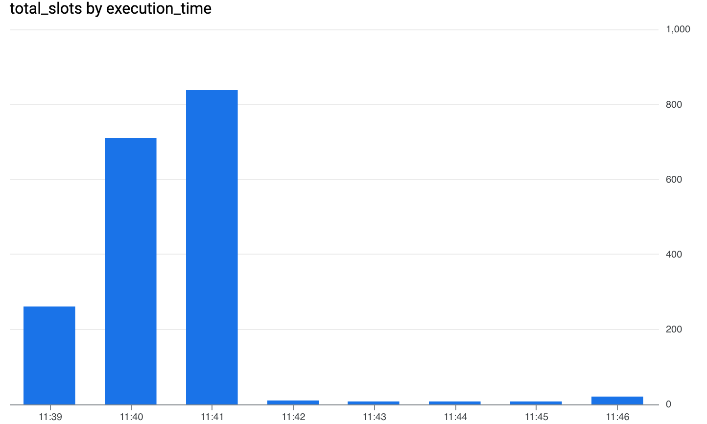
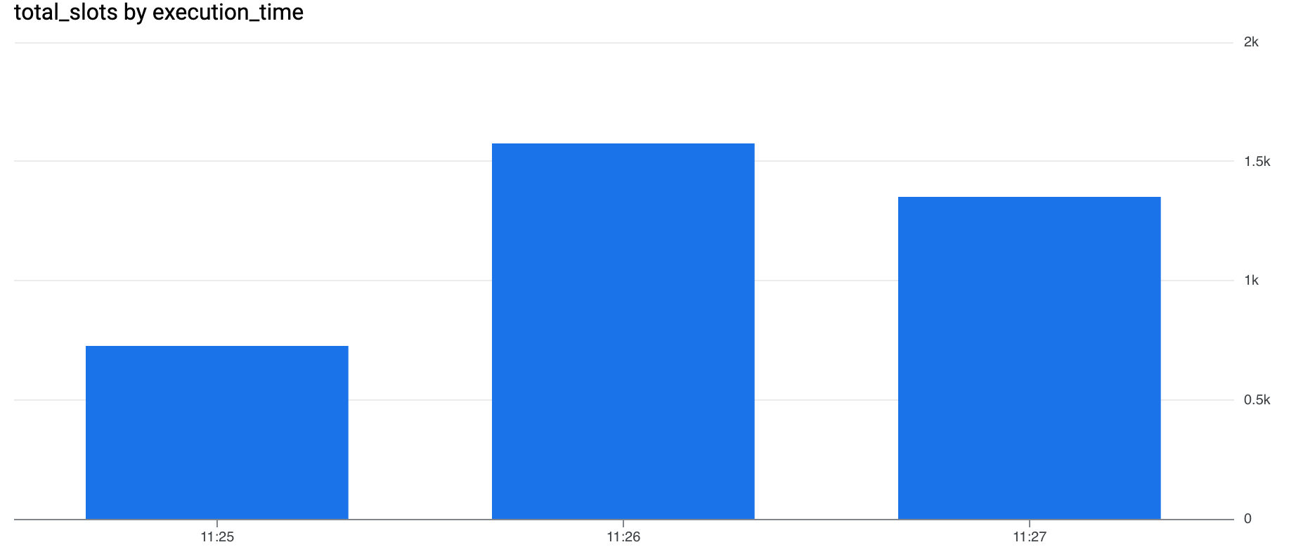
The INFORMATION_SCHEMA.JOBS_TIMELINE table gives us a granular view of slot allocation over time: right at the start, BigQuery allocated over 800 slots to the job, and the process was automatically scaled down. The query cost around 20 cents, a pretty solid deal.
SELECT
    FORMAT_TIMESTAMP("%H:%M", period_start, "UTC") as execution_time,
    ROUND(SUM(period_slot_ms)/(1000*60)) AS total_slots,
FROM `mfg-internal-demo`.`region-us`.INFORMATION_SCHEMA.JOBS_TIMELINE
WHERE job_id = "bquxjob_555c4994_19386e173e8"
GROUP BY execution_time
ORDER BY execution_time;
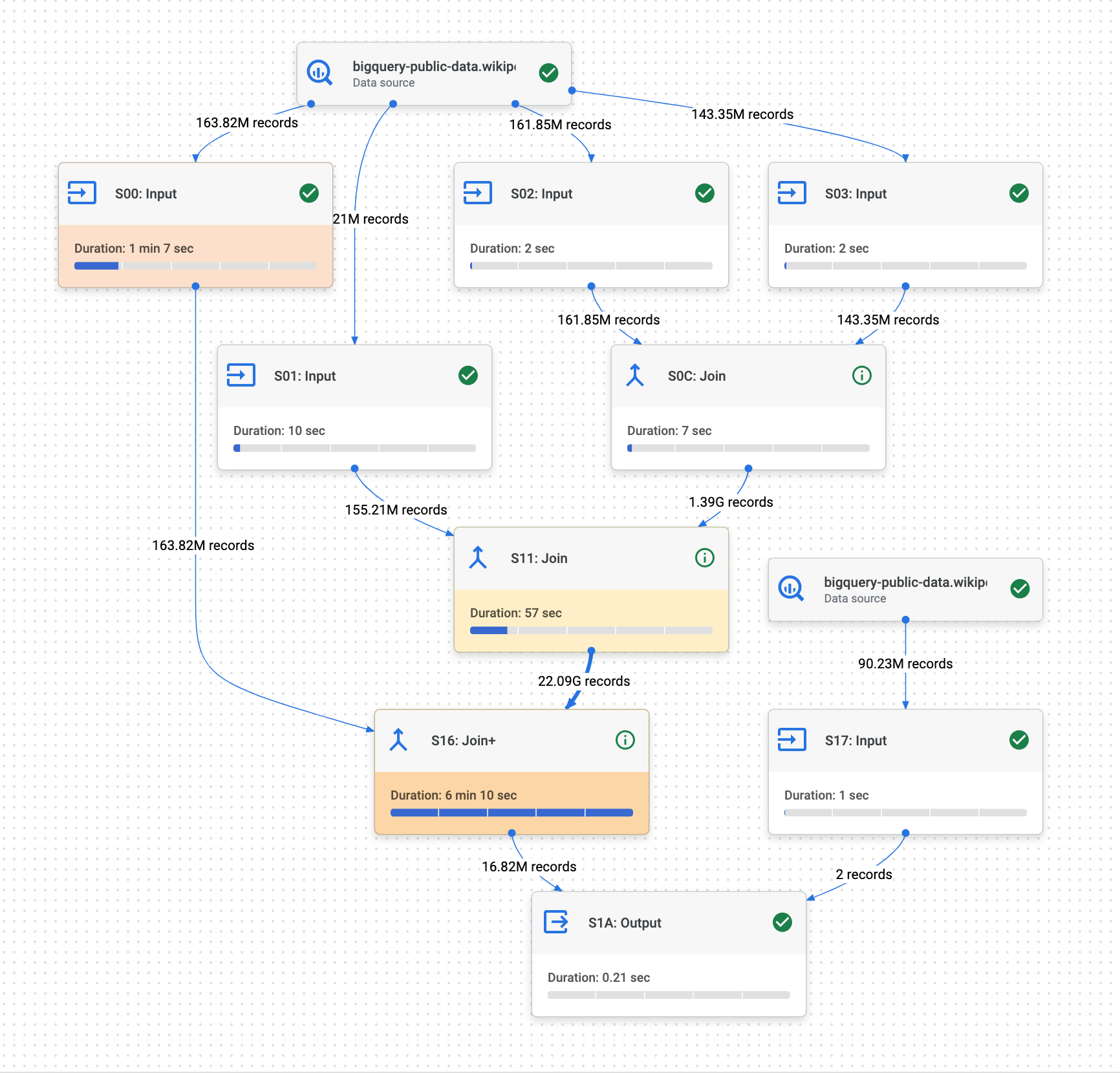
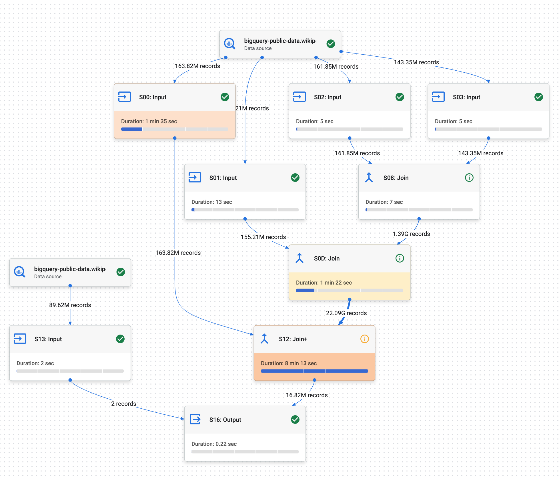
The query plan gives us insights into the steps performed by BigQuery, with various metrics associated with each step. It’s an essential tool to understand contention points and where to begin optimization.
Running the query capacity-based
To compare cost and execution time, let’s run the exact same query on our 200 slots reservation that we previously set up. As detailed below, when running on the reservation setup, the query takes about 14 minutes to complete.
| Duration: 9min 52s | Bytes shuffled: 1.31 TB |
| Slot time consumed: 1 day 6 hr | Bytes billed: 31.02 GB |
| Slot milliseconds: 108043988 | Query price: $2.4 |
| Edition: Enterprise | Location: US |
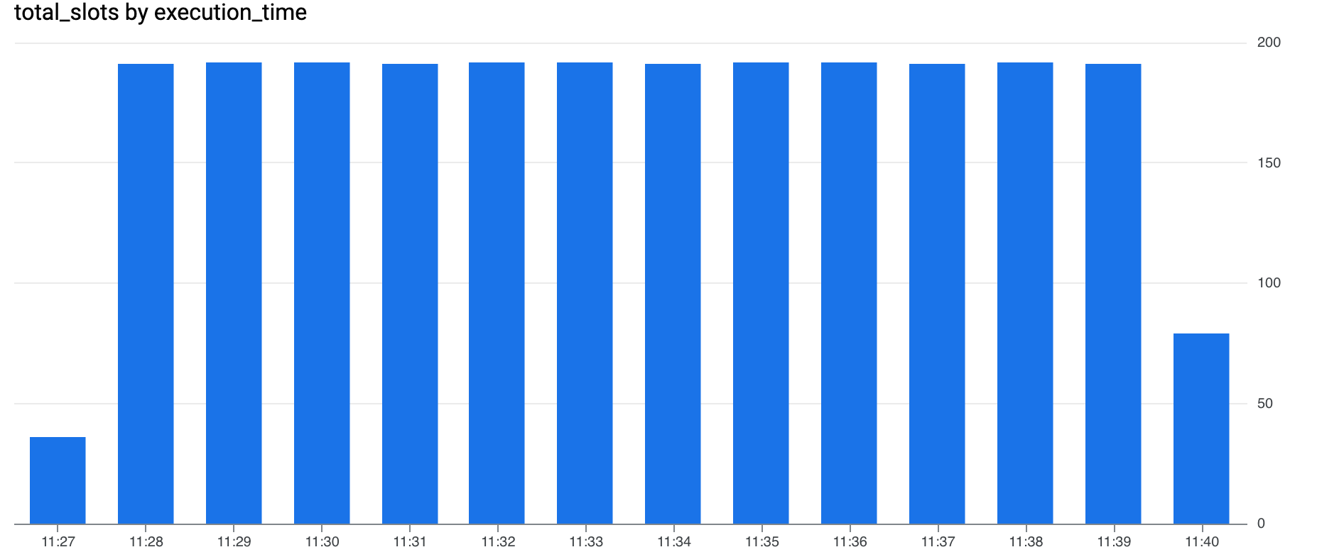
Using the INFORMATION_SCHEMA.JOBS_TIMELINE once again, we can get a fine-grained view of the evolution of allocated slots, which automatically scaled up to 200 slots and then decreased once the job was completed. At $0.078 per slot per minute, the job cost around $2.4. This query lasted ~35% longer and cost 12 times more than the previous one - not much to say here, as expected: this use case is better suited for on-demand. If you have a few queries to run, no need for the big gun, just go on-demand.
SELECT
 FORMAT_TIMESTAMP("%H:%M", period_start, "UTC") as execution_time,
 ROUND(SUM(period_slot_ms)/(1000*60)) AS total_slots,
FROM `fsa-bqe-tests`.`region-us`.INFORMATION_SCHEMA.JOBS_TIMELINE
WHERE job_id = "bquxjob_7f0b2bc7_193881b720f"
GROUP BY execution_time
ORDER BY execution_time;

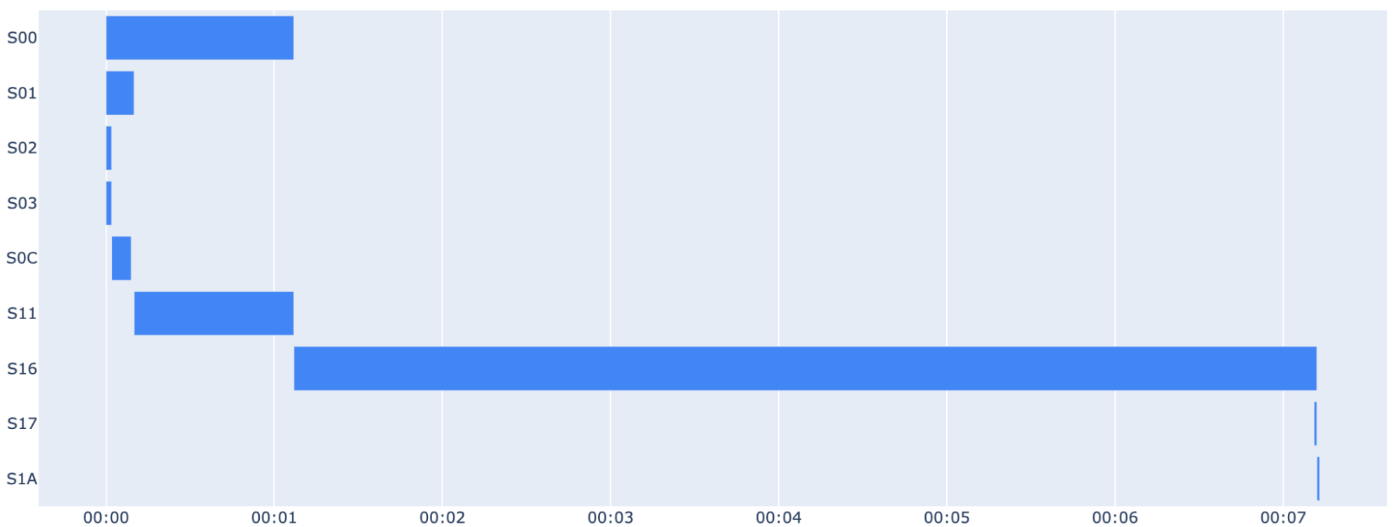
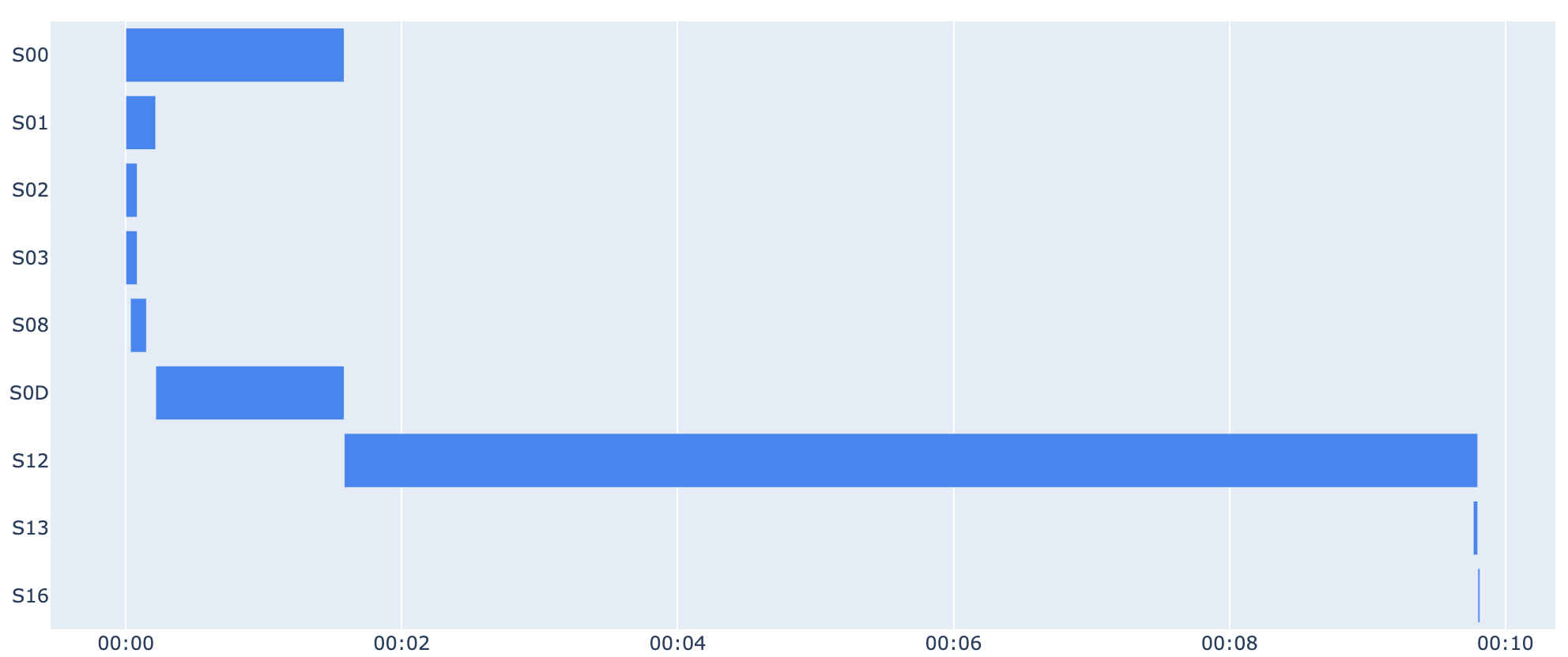
Just like before, the query plan provides detailed insights into each step performed by BigQuery, highlighting the slowest steps and potential bottlenecks (the join during S12 in our case, which accounts for more than 80% of the total query time).
For infrequent, complex queries like this one, the on-demand model offers significant cost savings compared to a reserved capacity model. While the reserved capacity provides consistent performance, it’s not always the most economical choice, especially for ad-hoc or less frequent workloads. Let’s shift in perspective as we delve into a second use case, where the benefits of a reserved capacity model become clear.
Second use-case: let’s open the valves
The second query is similar but smaller. Let’s build a small Python script to easily run it many times - each query is scanning around ~18GB.
import random
import datetime
from google.colab import auth
from google.cloud import bigquery

def random_month():
  return f"{(random.randrange(12) + 1):02}"

projects = {'mfg-internal-demo' : [], 'fsa-bqe-tests': []}
run_id = f"run_{datetime.datetime.now().strftime('%d%m_%H%M')}"

for project in projects.keys():
  client = bigquery.Client(project=project)
  job_config = bigquery.QueryJobConfig(use_query_cache=False)
  for _ in range(100):
    first_month, second_month = random_month(), random_month()
    sql = f"""
        WITH
        first_month_views AS (
          SELECT * FROM `bigquery-public-data.wikipedia.pageviews_2024`
          WHERE TIMESTAMP_TRUNC(datehour, DAY) = TIMESTAMP('2024-{first_month}-01')
        ),
        second_month_views AS (
          SELECT * FROM `bigquery-public-data.wikipedia.pageviews_2024`
          WHERE TIMESTAMP_TRUNC(datehour, DAY) = TIMESTAMP('2024-{second_month}-01')
        ),
        average_views AS (
          SELECT
            first_month_views.title,
            SUM(first_month_views.views + second_month_views.views ) / 2 AS average_views
          FROM first_month_views
          INNER JOIN second_month_views  USING (wiki, title)
          GROUP BY title
        )
        SELECT title, average_views.average_views
        FROM average_views
        INNER JOIN `bigquery-public-data.wikipedia.wikidata` AS wikidata
        ON wikidata.en_wiki = average_views.title
        WHERE wikidata.en_label = 'Google';
    """
    query_job = client.query(sql, job_config=job_config)
    job_id = query_job.job_id
    projects[project].append(job_id)
Let’s also store each job_ids to reuse it later and to facilitate analysis:
def create_insert_query(table_name, data):
  structs = [
      "STRUCT('{}' AS project, '{}' AS job_id)".format(project, job_id)
      for project, job_ids in data.items()
      for job_id in job_ids
  ]
  sql = """
  CREATE OR REPLACE TABLE `bqe_tests.{table_name}` (
      project STRING,
      job_id STRING
  );
  INSERT INTO `bqe_tests.{table_name}` (project, job_id)
  SELECT * FROM UNNEST([
      {structs}
  ]);
  """.format(table_name=table_name, structs=',\n'.join(structs))
  return sql

client = bigquery.Client(project='mfg-internal-demo')
query_job = client.query(create_insert_query(run_id, projects))
Running the queries on-demand
Just like before, let’s start with on-demand. As this time we are running multiple queries, I don’t have a global results table to display so let’s go straight to the INFORMATION_SCHEMA
SELECT
    FORMAT_TIMESTAMP("%H:%M", period_start, "UTC") as execution_time,
    ROUND(SUM(period_slot_ms)/(1000*60)) AS total_slots,
FROM `mfg-internal-demo`.`region-us`.INFORMATION_SCHEMA.JOBS_TIMELINE
INNER JOIN (
    SELECT job_id FROM  `bqe_tests.run_0612_1125`
    WHERE project = "mfg-internal-demo"
) AS run USING (job_id)
GROUP BY execution_time
ORDER BY execution_time;
Let’s calculate the cost before jumping to a conclusion
SELECT (SUM(total_bytes_billed)/(10e8))*(7.5/1000)
 FROM (
  SELECT
  job_id,
  period_start,
  period_slot_ms,
  total_bytes_billed
  FROM `mfg-internal-demo`.`region-us`.INFORMATION_SCHEMA.JOBS_TIMELINE
  INNER JOIN (
    SELECT job_id FROM  `bqe_tests.run_0612_1125`
    WHERE project = "mfg-internal-demo"
  ) AS run
  USING(job_id)
  WHERE  state = "DONE"
 )
All the jobs completed in 2min 33s for a total of 14$, still acceptable but costs will increase linearly if the number of queries continues to grow. This potential issue can be mitigated by defining quotas (if it’s acceptable to pull the plug) and/or budget alerts. Now, let’s see what happens if we run the same script on the reservation.
Running the query capacity-based
Here is what we get after running the script on the 200-slots reservation.
SELECT
FORMAT_TIMESTAMP("%H:%M", period_start, "UTC") as execution_time,
ROUND(SUM(period_slot_ms)/(1000*60)) AS total_slots,
FROM `fsa-bqe-tests`.`region-us`.INFORMATION_SCHEMA.JOBS_TIMELINE
INNER JOIN (
 SELECT job_id FROM  `bqe_tests.run_0612_1125`
 WHERE project = "fsa-bqe-tests"
) AS run USING (job_id)
GROUP BY execution_time
ORDER BY execution_time;
At first glance, it took longer but let’s have a look at the cost:
  SELECT SUM(price)
  FROM (
    SELECT
      FORMAT_TIMESTAMP("%H:%M", period_start, "UTC") as execution_time,
      ROUND(SUM(period_slot_ms)/(1000*60)) AS total_slots,
      (ROUND(SUM(period_slot_ms)/(1000*60)) *0.078/60) AS price
    FROM `fsa-bqe-tests`.`region-us`.INFORMATION_SCHEMA.JOBS_TIMELINE
    INNER JOIN (
      SELECT job_id FROM  `mfg-internal-demo.bqe_tests.run_0612_1125`
      WHERE project = "fsa-bqe-tests"
    ) AS run
    USING(job_id)
    GROUP BY execution_time
    ORDER BY execution_time
  )
While slower (approximately 12 minutes), running the jobs on the reservation resulted in a significant cost reduction: $3.14, 4.5 times cheaper than on-demand. This illustrates how reservations can optimize spending for high-volume workloads, offering a compelling balance between cost efficiency and acceptable performance. Furthermore, committing to a quantity of slots for one or three years can yield even lower hourly slot prices for the baseline, with discounts of 20% and 40% respectively.
We could gradually increase the number of queries, but you get the point: for infrequent, complex queries, on-demand offers cost-effectiveness, performance and simplicity. However, as query volume and frequency increase, a capacity-based approach becomes increasingly attractive financially.
Conclusion
By starting with on-demand and transitioning to an Edition as your needs evolve, you can optimize your BigQuery bill without sacrificing performance. Remember that both models can coexist, allowing you to tailor your approach to different workloads and achieve the ideal balance between cost and performance. In practice, our clients often find success by adopting a hybrid approach, leveraging both on-demand and capacity-based models. While individual queries or use cases might be best suited for one or the other, at the organizational level, a combination of both delivers optimal cost efficiency and performance.
Ultimately, BigQuery offers the flexibility to adapt to your specific needs, whether you’re running a single complex query or handling a continuous stream of requests.
🚕 vs 🚗
Above all, keep in mind:
- On-demand is like taking a taxi, you only pay for the distance traveled, no need to own a car or worry about maintenance. It’s perfect for infrequent trips.
- Editions are like renting a car, you pay a monthly fee regardless of usage, you can customize your car as you wish and it just makes more sense if you drive a lot!
Just like choosing between using a taxi and renting a car depends on your needs and driving habits, choosing between on-demand and Editions depends on your BigQuery usage patterns.